Interpretation of Topology Optimization

Browsing through studies regarding design, it can be found that the integration between form and structure always remains as a popular topic. Tracing back to the past, some architects has adamant structural sensibility when producing a masterpiece. Among them, Antoni Gaudí (1852–1926) was a Master Builder. It was him who originally used the concept of catenary arches, which successfully combines the structural design with the architectural design. For example, applied the hanging models into the design of the church at the Colònia Güell [Figure1], the structural problem of which cannot be solved directly. Therefore, he used iteration. The model is modified by the loads until it adopts a shape approximate to the equilibrium state. The way he visualize the result is also interesting. By drawing on the photograph of the model, he tried to show the volume of the model [Figure2](Santiago Huerta, 2006).

Designing form in an “optimal” way arouses a considerable enthusiasm in a wide variety of applications. It has become increasingly important due to sustainable development, the limited resources and technological competition. Structural Optimization aims to make a structure to achieve the best performance on one or more such criteria. It can be divided into three categories: size, shape and Topology Optimization with each of them target on different types of parameters. Comparing the other two, Topology Optimization (TO) offers much more freedom for a designer to create totally innovative and efficient conceptual designs (Huang X and Xie M, 2010).

There are two types of TO, namely discrete or continuous types, which mainly depends on the type of the structure. For discrete structures like trusses and frames, TO is to figure out the optimal spatial order and connectivity of the structural members. This area has been largely developed by Prager and Rozvany. On the other hand, TO of continuum structures is to search the optimal designs through pinpointing the best locations and geometries of cavities in the design space (Huang X and Xie M, 2010). This paper presents an analysis over the TO of continuum structures. Numerous methods for Topology Optimization of continuum structures have been explored extensively after the landmark paper of Bendsøe and Kikuchi (1988). Most methods rely on finite element method (FEM) to optimize material by referring to a defined set of criteria. In this context, the optimization procedure is to find the topology of a structure through confirming whether there should be a solid element or void element at every point in the design field (Huang X and Xie M, 2010). In recent years, TO is widely used. Its applications range from nano-science to aeroplanes. However, it has been barely applied in architecture.

This design report mainly focuses on translating the data from TO into design. The organization of the paper is presents as follows: In section 2, some optimal nature structures are discussed. Then, in section 3, an analysis over the background of TO and some methods is presented. In section 4, the author reviews state of the art and the limitations of TO. In section 5, one of the interpretation of TO using a chair design as the case study is provided. Finally, the author evaluates the whole process of entire project.

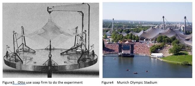
Almost every creature has been exposed to a tough competition, in which they either strive for energy or for living space in nature. Only the design which fits the nature with high reliability and minimum consumption of materials and energy will survive (A. Baumgartner, L. Harzheim and C. Mattheck, 1992). In nature, the form and the structure are integrated because they are fused together during the evolutionary processes of biological forms. Take the bubbles as an example, they are structures made from liquids. When it was given a set of fixed points, soap film will spread naturally between them to offer the smallest possible surface area. According to Ball (1999), bubbles tend to minimise the area of their surfaces as all physical systems and hence to reach their most equilibrium state. This structure inspired architect like Frei Otto. He made use of soap films stretched across wireframes to plan the curves of his membrane structure [Figure3]. From the 1950s, he designed many tent-like shapes whose curvature is calculated to minimise surface area [Figure4].

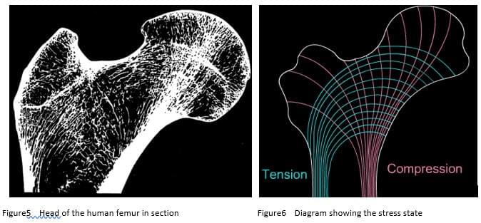
Bone is the best sample in this research. It is a “smart” material, being remarkably strong and having lightweight. In his book, On Growth and Form, D’Arcy Thompson introduced the idea that bone adapts by reacting to load induced mechanical deformation. Firstly, taking the long bone of a bird’s wing as an example, Thompson points out the hollow and tubular structure which carries little weight, can be stiff enough to support the “powerful bending moments”. It supports the bird’s wing in flight without breaking. Secondly, bone is also a living material. It continuously renews itself by replacing old or damaged component with new one (S. J. Mellon and K. E. Tanner.2012) . Thirdly, bone reacts to its mechanical environment by increasing or decreasing the amount of material. Before talking about bone, Thompson once (1917) discussed that “In all the structure raised by enginer, in beams, pillars and girders of every kind, provision has to be made, somehow or other, for strength of two kinds, strength to resist compression or crushing, and strength to resist tension or pulling asunder.” When it comes to the upper section of the femur [Figure5], the structure and distribution of trabecular and cortical bone efficiently reflected the lines of stress (both tensile and compressive) when the bone acts as supporting structures. [Figure6]. It is Thompson who reveals the essence of the depiction of bone strength since the mechanical adaptability of bone had been debated for many years. This example perfectly illustrates how nature finds its way to design the structure efficiently, which human can always learn from it.

3.1 Background

The researcher has developed many computational Optimization tools to make up the drawbacks of the availability of infinite computing. Structural Optimization can be divided into three distinct branches with each targeting on different types of parameters: topology, size and shape Optimization [Figure7]. The techniques target either only topology or only size and shape Optimization, with few exceptions that try to formulate the problem in an integrated way.

According to Katsuyuki Suzuki and Noboru Kikuchi (1991), size Optimization is often used for either finding the optimal sizes of cross section of frames and trusses or calculating the optimal thicknesses of shells since most of the aeronautical applications are based on frame structure with shell reinforcement. With this method, the shape or connectivity of members may not change. However, they may be removed during the process. This is earliest and easiest approach to promoting structural performance. In other cases, most of the structure designs of different parts of machines need to be optimized in their shape because they rely heavily on their geometric presentation. Shape optimization is based on the form of the initial material layout in a domain. It allows the changes in the boundary of geometry to obtain an optimal solution. In this case, the optimization can reshape the material inside the domain but still retains its topological properties. To sum up, size and shape optimization cannot change the structural topology during the optimization process. However, the choice of the proper topology of a structure in the initial conceptual stage is of great importance as it determines the efficiency of the final result.

Topology optimization is introduced to overcome the limitations discussed above. It is the most general type of structural optimization, offering an initial model that can be fine-tuned afterwards with shape and size optimization. The purpose of TO is to get the optimal “lay-out” of the structure within a specified domain. In this case, the lay-out of the structure includes data on the topology, shape and the size of the form while the material distribution method allows for formulating all three problems at the same time (Bendsoe M P, Sigmund O, 2013). In this scenario, the size, the shape and connectivity of the form are unknown. Instead, the loads, the supporting conditions and the space, which need to be designed, are the only information known to the designers.

Another potential advantage of TO is that it is truly generative. The designer only needs to apply a set of parameters (boundary conditions, the loads, and the target, material type, weight restrictions, etc.) to the algorithm (in this case is TO). The system then does its job and finally hits the goal. The goal here is optimizing the material for a defined set of criteria. This whole process is a bottom-up and process, making it possible for designers to generate novel products. Different from traditional design, the role of the designer is not to manipulate the designed artifact directly but to be involved in creating or modifying the rules that are applied to produce the result autonomously.

3.2 Topology Optimization method

As stated above, TO has great Optimization potential since it is used in the initial phase of the design. During the past years, substantial progress has been achieved in the development of TO, especially by means of FEM, which is introduced by Richard Vourant in 1943 to figure out solutions for partial differential equations. It is also referred as finite element analysis(FEA). In this context, the geometry of the design domain is subdivided into smaller elements that are interconnected at nodes. Therefore, the entire domain, which is filled with elements without overlaps, is analyzed for functional performance. After applying boundary conditions and loads to the part, the resulting finite element equations are solved accordingly (Ramana M. Pidaparti, 2017). FEA is widely used in many areas of research, including biomedical, mechanical, civil, aerospace researches, etc. When it comes to TO, “The typical approach to plane or volumetric structures Topology Optimization is the discretization of the problem domain in a number finite elements and the assignment of full material, partial material or lack of material to each element, in an iterative scheme converging to the optimal material distribution inside the domain.” (Razvan CAZACU and Lucian GRAMA, 2014). A short review of the most common methods for TO is presented in below.

3.2.1 Solid Isotropic Material with Penalization (SIMP)

The SIMP method was proposed by Bendsøe (1989). When the design domain is discretized into specific elements, the SIMP method is based on the assumption that every element contains an isotropic material with variable density. The design variables refer to relative densities of the element. The power-law interpolation scheme then penalizes the intermediates to get the result with 0(void)/1(solid) material distribution (Huang X and Xie M, 2010). This techique is used to evaluate the material density distribution inside the design volume that minimizes strain energy for a preset structure domain. (Razvan CAZACU and Lucian GRAMA, 2014). For more information about SIMP, the readers can refer to the text book by Huang and Xie [11].

3.2.2 Evolutionary Structural Optimization (ESO)

ESO gets the optimum design by removing the lowest stressed material from the preset domain. This method is similar to SIMP as they work with a discrete design space. However, this one is a “hard-kill” approach, meaning that every element in the design volume has a density of either 0 (void) or 1 (Solid) (Razvan CAZACU and Lucian GRAMA, 2014). The structure is re-analyzed to figure out the new load paths each time elements are killed. This procedure continues until all the elements left support the same maximum stress. Apparently, the computational cost of this method is a significant problem. Bidirectional ESO (BESO)was developed to improve the efficiency. This method involves removing under-stressed material and simultaneously adding material to where the structure is over-stressed. Additionally, BESO allows designers to handle multiple loads for both 2D and 3D structures (Eschenauer H A and Olhoff N, 2001).

3.2.3 Soft Kill Option (SKO)

SKO is a soft-kill method, using a finite element grid and permitting the elements to have fractional material properties, which is like SIMP method does. Different from SIMP, SKO uses fractional elastic properties instead of fractional densities to represent how much material is needed. Moreover, it is also similar to the BESO method, which iteratively adds and removes elements to the model through their stress state. Moreover, SKO uses stresses as Optimization objectives. The purpose is to seek the result that gives a uniform distribution of the stresses (Razvan CAZACU and Lucian GRAMA, 2014).

3.3 Design tools

During recent years, there are more and more design tools for structural optimization become available to students, architects, engineers, etc. However, TO techniques are still beyond the reach of most designers because of the complexity of algorithms as well as the lack of friendly used software. In this paper, the author mainly use MillipedeTM which implements the BESO approach. This plugin for grasshopper is developed by Michalatos Panagiotis and Kaijima Sawako (Panagiotis and Sawako, 2014). It is a Grasshopper™ component which is applied in the analysis and Optimization of structures. At the core of this component is a library of very fast structural analysis algorithms for linear elastic systems. The library contains its own Optimization algorithms based on Topology Optimization (Panagiotis and Sawako, 2014). Millipede requires users to adjust settings manually for each structure. This tool makes it hard to create an automated system around Millipede: there is little ability to automate the decision-making system so that decisions about support types, material types, connection points are automated for designers. Rather, designers need to make these decisions by themselves manually. That is adequate and useful for specific design projects in which specifications are known. However, it limits the atomization ability in creating a general-purpose truss design tool (Makris M P, 2013).

Add paragraph text here.

4.1 State of the Art

As shown below[Figure7], the Bone Chair designed by Joris Laarman is based on the generative process of bones. When bones grow, areas not exposed to high stress develop less mass while sectors that bear more stress develop added mass for strength. The working principle of the chair is likewise. He used CAO (computer-aided Optimization) and SKO (soft kill option) Optimization software to produce the form of the chair rather than applying the software to a pre-existing gemetory. The whole design process is a bottom-up approach and is aesthetically innovative (Bittiner J, 2008).

The first applications of modern shape and Topology Optimization techniques in architecture have been presented by Sasaki and his co-workers. Qatar National Convention Center was designed by referring the Sidrat al-Muntaha, an Islamic holy tree. "The tree is a beacon of learning and comfort in the desert and a haven for poets and scholars who gathered beneath its branches to share knowledge," said Sasaki. However, the fact is that the tree-like structure was not designed to look like Sidra Tree. Instead, it was purely mathematical calculation. It was made to support the external canopy in an ideal engineering way. The main façade adopts the Bi-directional Evolutionary Structural Optimization (BESO) method. The structure evolved from an initial deck with simply legs into the final form in which it is presented to the public. The interpretation from TO in this case is quite successful in terms of aesthetics. The architect was able to design a novel and organic form that touched the client. On the other hand, although this design strives for a high sustainability level. It is doubtful if this tree-like structure is the most material efficient solution. The construction of this masterpiece is a daunting task. Besides, it is quite costly by means of present techniques. According to Obbard, the steelwork specialist, the building structure was constructed upside down from roof deck to foundations using Macalloy bars. Regarding the deck took considerable loads and the angle of the branches was extreme, the tree structure had to be extremely strong: as Obbard said, ”This is the most complicated piece of steelwork I’ve ever seen”.

4.2 Limitations

As discussed above, TO can be an initial phase towards the production of efficient designs. However, it also has limitations. Firstly, the result got from TO cannot be used directly but need to be interpreted. This process can be tough, especially in the case of volumetric structures, in which the designer needs to build models as close to the ones done by the Optimization routines (Cazacu R and Grama L, 2014). Secondly, the practical realisation of the obtained results. The goal of TO is to find the optimal design for the preset criteria, not to make an affordable or feasible model to fabrication using traditional methods. In recent years, by using Additive Manufacturing (AM), these geometries are now feasible to manufacture. This method, for now, is mostly restricted to art works because it requires the advanced fabrication techniques which are quite costly.

5.1 Overview

This research paper aims to interpret Topology Optimization of design while simultaneously considering fabrication constraints. In precise terms, this work focuses on the translation of data extracted from analysis and Optimization of structures into aesthetic form. In terms of fabrication, the integration of TO and 3D lattice printing has great potential to achieve this objective.

Lattice structure is commonly used in architectural design as it is one of the strongest types of structure and can be applied to different geome­tries. By using a single cost-saving material, it is possible to create a structure that is dense and strong in parts (for load-bearing walls), lightweight and penetrable in others (for non-load bearing walls), and near-transparent in others (to permit the inflow of natural lighting). In the case of digital fabrication, 3D lattice structures offer versatility of form and the possibility of utilisation of a standard module for production. This means that materials can be distributed spatially in an efficient manner. This advantage provides the capability to fabricate large scale structures.

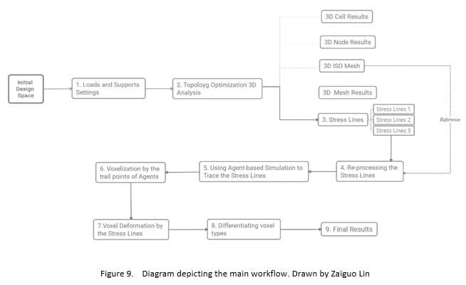
Figure 9 shows the main workflow of this research. This work uses the design of a chair as example to illustrate the whole process. Although the chair is a simple object, it is also a functional structure designed to accommodate one person. It is structurally as complex as architectural design. In the beginning, the designer needs to input parameters such as the boundary conditions, the loads, the support regions, etc. After applying TO to the 3D structure in the design platform (Millipede), the outputs are analysed. Four principal methods are developed to translate the data into the final results. More details are discussed in the following sections.

5.2 Load and support conditions

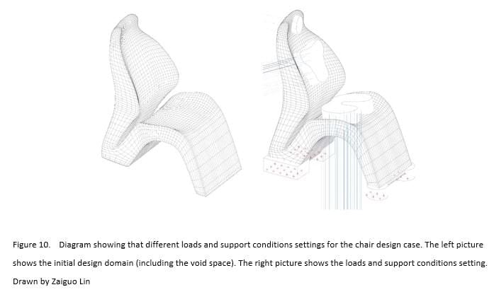
As an initial step, the role of the designer in this stage is also important as discussed before. The designer is required to make decisions about the material types, self-weight factor, connection points, support regions, load regions, force directions, etc. In terms of the target geometry, the designer also needs to find the balance of how much should he design for the prototype. If he designs too much, TO will lose its power: the analysis process tends to be Shape/Size Optimization. In the Millipede framework the boundary conditions for the TO are to be defined as abstract geometrical objects. Furthermore, a model component called system builder which regulates the resolution of the individual finite elements is required. Millipede only provides the resolution along the x axis. The resolution of other axis is calculated automated within bounding box of all defined brep regions. The higher the values, the finer grained the material distribution can be. But this parameter can dramatically increase the time and memory requirements of the solver. Apart from this, the numeric control of the total material volume used allows different results from the Optimization process. In the project example of chair design, it is possible for the designer to apply multiple load cases to the domain, the main loads include the seat loads, the back loads and the head loads and these are set by the designer. All the load forces have their own directions and they all result in the support regions that form the legs [Figure 10].

5.3 Translating the data

After the iterative form-finding process, the structural data is stored as an individual FE-cell container. Millipede provides several outputs from 3D Topology Optimization[Figure 11]. Figure11.1 shows the contours along surfaces of constant material density. Adjusting the contour value, the user can decide the density levels at which contours are drawn. This output is the most widely used among the designers as it offers direct mesh geometry. Figure11.2 illustrates the material distribution and stress as a series of horizontal meshes cutting though the region of the domain. The node results as figure11.3 showed visualize the locations and displacements of all nodes. Figure 11.4 shows the results for all volume elements in the system. The output in Figure 11.4 shows the stress lines in the design domain. In the context of 3D structure, Millipede offers three types of stress lines which are showed separately from figure11.4.1 to figure 11.4.3. Additionally, by selecting the seed points in this solver, the designer can choose to visualize the stress lines in a certain region.

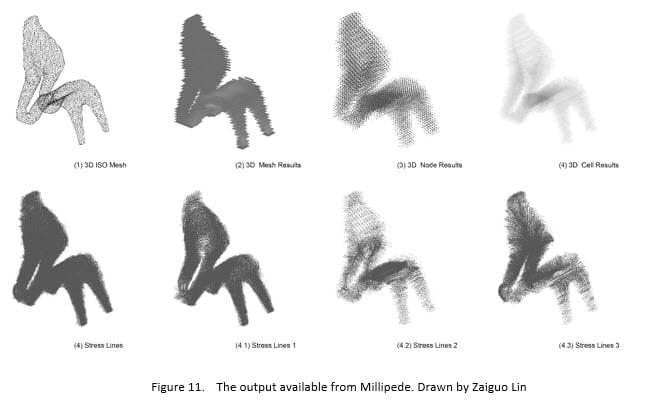
Amongst the available output from Millipede are the principal stress lines which are pairs of orthogonal curves naturally encoding the optimal topology since they indicate the trajectories of internal forces (Tam K M M, 2015). To be more precise, principle stress lines are numerical translations of the principal stress directions over a structural body.

The construction of stress lines starts with the decomposition of a structure into infinitesimal elements to decide the state of stress at each point, which is characterised by two normal components and a shear component (Tam K M M,2015). The state of stress remains unchanged when rotating the element. However, the stress components correspond to the transformed orientation. To be precise, the principal stress directions are the normal stress components where the shear stress is zero and the normal stresses are maximum. Once the principal stress directions across a structure are determined, these vectors are projected as lines that form the principal stress lines.

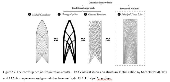
According to Chen and Li (2010), stress line results are entirely influence by the geometric attributes of the design domain including the locations and directions of loadings, the positioning and degree of fixing of supports, and the boundary shapes, regardless of the scale of the material properties, applied forces or object dimensions. Finally, the optimal geometry for a design domain is included in the principal stress field [Figure 12].

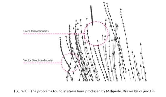
Although stress lines have the potential to provide a direct and provocative approach to Optimization, their application in design has been limited due to lack of parameterization of the process for interpreting stress lines (Tam K M M, 2015). The Millipede interface for generating stress lines is typically concerned with the visualisation of stress flow instead of the realisation of practical design applications. The stress lines produced cannot be directly used for design but need to be reprocessed because of the force discontinuities and vector direction disunity [Figure 13].

In the Millipede interface, stress is measured as axial, shear, and bending varieties [Figure 11]. Apart from these three forces, there are forms of stress and strain such as torsional forces and changes in temperature which can act on the structural body. Translating all these forces could lead to complex results that are difficult to analyse. Due to the load settings in this chair design, this work deals exclusively with the axial stresses since these represent the main forces. Before interpretation, the designer has to handle the raw stress lines from Millipede manually to make them usable. In the next step, four methods are developed to transform the data into an object that can be manufactured, based on the selected stresses. The first is the application of an agent-based modelling method to re-simulate the axial stresses from the load regions to the support regions. Although using the reprocessed stress lines directly is the most straightforward way to capture the data, it will give the designer more freedom to explore different results when applying agent-based simulation. This is followed by achieving high resolution with voxelization by the trail points of the agent. The third method involves deforming the normal voxels according to the stress lines. Finally, the types of Voxels can be differentiated according to the attractors. These are discussed in detail as follows.

5.3.1 Simulating the stress-flow

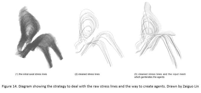
In order to simulate the stress force flowing from the load regions to the support regions, the first step is to set the input data. In the chair design, the 3D ISO mesh [Figure 11.1] generated from Millipede is used as a reference to clean the stress lines [Figure 14.2]. As discussed earlier, it is necessary to unify the direction of the stress vectors. Apart from this, the agents extracted from the mesh points of the seat and the back surfaces are created by the designer [Figure 14.3].

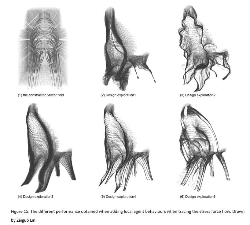
Instead of allowing the agents to simply trace the processed stress vector, several explorations are developed that all produce different results. As Fiugre15.1 shows, the first step is to construct an entire new vector field according to the stress vectors. In this case, the domain of the vector field is set by 65 cm along the X axis, 100 cm along the Y axis and 120 cm along the Z axis. The resolution here is 1 cm and it has an interrelationship with the density of the processed stress lines. After setting up the vector field’s data structure, the designer computes the vectors according to the input stress lines in the field itself. The basic logic is to set up an influenced range A around the stress vectors. It is only inside the range A that the vectors are calculated to point to stress vectors. When it comes to the third step, inside range A, another variable that can be called influenced range B which is smaller than range A is introduced. The vectors inside range B are calculated to copy the directionality of the stress vector. Therefore, all the design proposals show in figure 15 is based on this scenario. In design exploration 1 [Figure 15.2], the agents simply follow the calculated vector field. Since the range A of influence is large in this case, the parameter is 30 cm while range B is 6 cm. The agents finally aggregate too much when they form the front legs of the chair and this makes the structure unstable. In design exploration 2 [Figure 15.3], the influenced range A is set at a much lower value (10 cm) while the range B remains 6 cm, and at the same time, Perlin Noise is applied when constructing the vector field. The final result shows the ecological form. In the case of design exploration 3 [Figure 15.4], the parameter of the influenced range A and range B is decreased (6 cm and 4 cm respectively) without applying Perlin Noise. The Alignment force is also applied in this case. The difference between design exploration 3 and design exploration 4 [Figure 15.5] is the influenced range. This can capture more detailed information about the stress vectors. Another type of agent is introduced in design exploration 5 [Figure 15.6] and this makes the whole system more complex than the previous cases. This approach goes a little too far for the translation of the stress data. From these cases, the exploration 4 is selected as the foundation for the second stage, since here the agents both capture the information about the stress vectors and display the local behaviours.

5.3.2 Voxelization by the trail points of agents

For now, the agent behaviour displayed above is only a flow of data. To make a structure, a transformation must happen into physical domain. Voxel computation has been used in recent archi­tectural research. 3D voxels are created to encapsulate the input point set. Each cube incorporates one or more data points inside its volume. The cubes are in fact the boundary forms of the points in the structure. By using the method of voxelization, the agent behaviour can be translated into geometry without loss of resolution. In this case, the designed voxel field domain is kept the same as the previous vector field (65 cm x 100 cm x 120 cm) and the size of each voxel is 1 cm. The basic logic to activate the voxels is using the trail points of the agents. Inside the field, each voxel is inactivated as default. Once the agents behaviour is decided, each voxel checks whether it contains any trail points inside its volume. It will be activated when finding any trail points stayed inside. To go to a further step as the designer developed, when a voxel finds there are more than a certain number of trail points inside the cube (e.g., Twenty), its neighbours also can be activated as will. With this logic, it is easy to understand that the voxelized geometry depends on the numbers and behaviors of the agents: their density, speed,velocity, etc. Figure 16 shows the explorations where a balance is found to achieve a continuous structure without losing the information from the agent behaviour .

5.3.3 Deformation algorithms

The ability to deform the regular voxel reveals the high performance of the lattice structure. In this project, several algorithms are developed to capture the direction of the stress lines [Figure 17]. To make readers easy to understand the deformation method, a simple scenario is set up: the author puts a series of stress vectors into the activated 2D voxels framework. The first exploration [Figure17.1] is that of compression. The influenced range of deformation needs to defined at the start. Inside the domain of influence, each voxel vertex finds the location of the closest attractor ( in this case it is the stress vector) and moves toward it. The distance moved depends on the distance to the attractors. The closer the voxel vertex is to the stress vectors, the more the distance moved. One of the disadvantages of this algorithm is that the closest vertex deforms too much and squeezes the attractor. The second strategy [Figure 17.2] captures the attractor’s direction. Inside the influence domain defined by the designer, each vertex finds the location of the closest attractor and copies its velocity. The closer ones move more, and the farthest ones do not move at all. The two algorithms developed above show a clear gap when the vertices are deforming. Starting from strategy 3 [Figure 17.3], a magnetic field is constructed according to the attractors. Strategy 4 [Figure 17.4] combines both compression and orientation effect. Two ranges of influence are set. Inside the first domain, the vertices move towards the vector fields. In the second range, which is smaller than the first, each vertex of the voxels inside the deformation range moves in the same direction as the attractor agents. Finally, to make the deformation smooth and possible to fabricate, the distance moved by each vertex is defined parabolically.

5.3.4 Combining different types of voxel

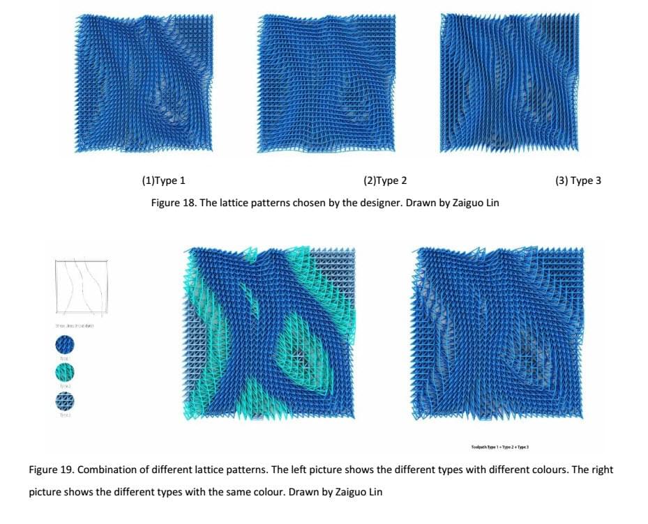
After deforming the regular voxels, the combination of different types of voxels also has the potential to meet different functional requirements. These different types of voxels could be different densities or different directions with the same den­sity. Figure 18 shows the result of deformation with three different lattice patterns chosen by the designer in a one-layer 3D voxelized patch. They have similar structural performance. The criterion for evaluating them is aesthetic. Figure 19 shows the logic of combining these three types. The designer set the rules to differentiate voxel types corresponding different lattice patterns by checking the distance from the activated voxels to the attractors. Type one captures directionality best and is placed within the first range.

5.3.5 Final Results

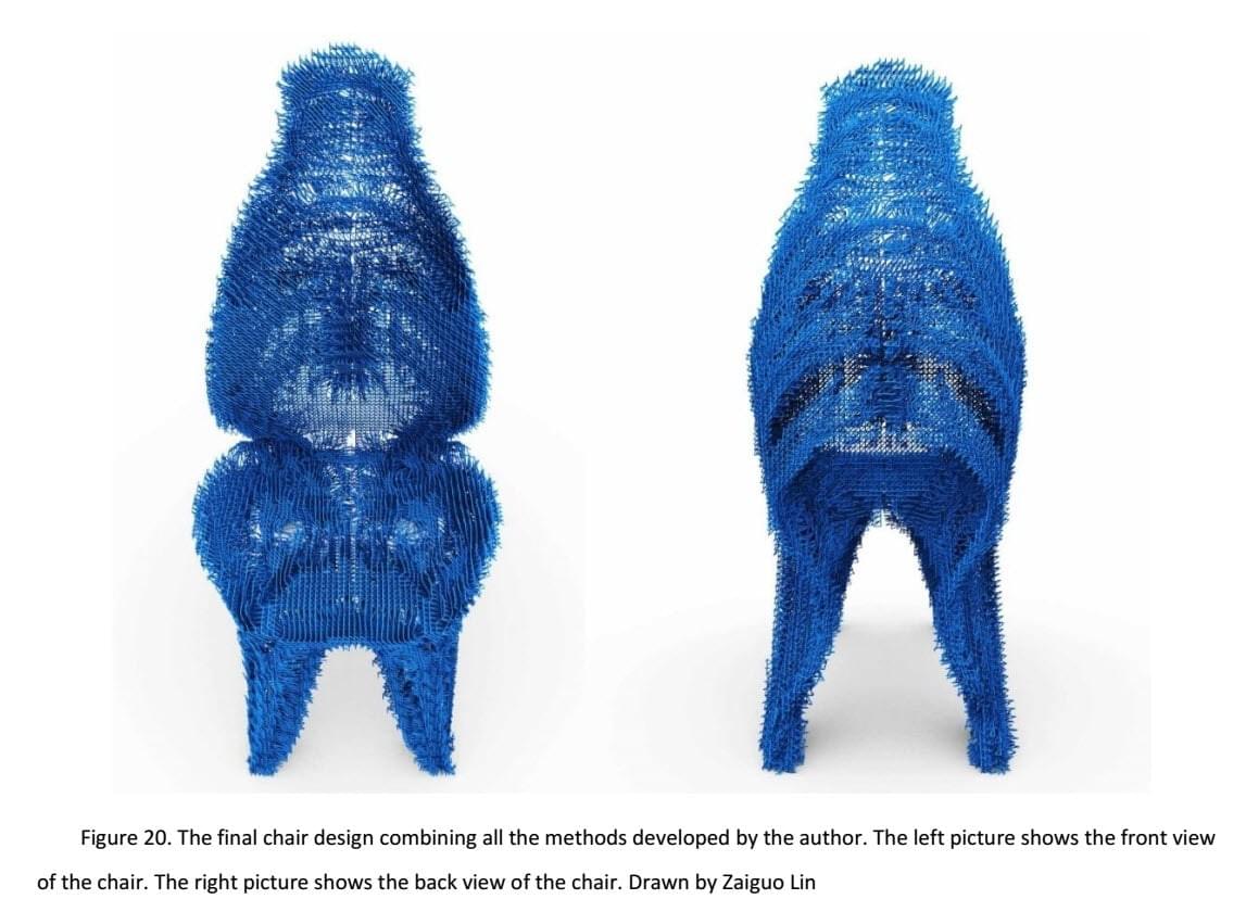
It cannot be guaranteed that combining best result of each methods developed above leads to the best design proposal. To be more precise, the methods are interrelated and interact on each other. Sometimes they even share the same parameters. Therefore, it is essential for the designer to find a balance when cooperating with all these methods. Figure 20 and figure 21shows the final proposal for the chair design combining all the methods. Although the deformation and differentiation of the lattice patterns according to the stress lines can intuitively improve the structural performance of the result, the criterion for evaluating it is the interpretation of the data as much as possible.

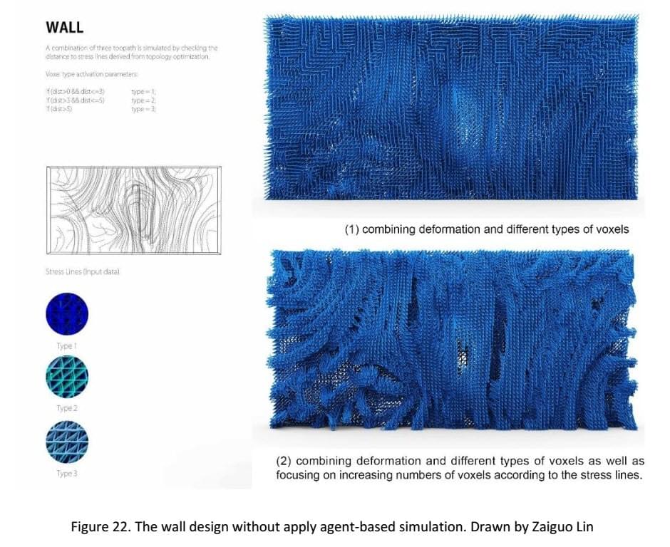
Additionally, It is also feasible to apply the methods separately or combine either two or three. The different strategies will give different results. For example, as Figure 22 shows, the wall design case applies the stress lines directly as the input data to deform and differentiate the lattice patterns.

6. Conclusion

This report starts with a popular theme, the integration between form and structure. The examples from nature keep inspiring the scientists, engineers, architects and so on. Natural ecosystems have a complex biological structure that most man-made environments do not have: they recycle their materials, permit change and adaptation, and make efficient use of ambient energy (J Frazer,1995). The introduction of Topology Optimization makes it possible for designers to get the optimal ”layout” of the structure within a predefined domain. Over the last decade, substantial progress of this technique has been achieved in many areas of research. With the rapid development of Additive Manufacturing, TO is becoming popular among designers and architects. In this paper, the short view about this technique is also introduced.

Additionally, the author draws inspiration from D’Arcy Wentworth Thompson’s book, on Growth and Form. He regarded the form not as a given, but as an outcome of dynamic forces that are developed by flows of energy and stages of growth (Sarah Bnonnemasion and Philip Beesley, 2008). This concept becomes increasingly possible to be achieved by the development of computer science. As a result, the attention of the architect is shifted from the visible, formal representation, to extend it into a domain of the invisible: the underlying logic and procedures (A Andrasek and D Andreen,2016). In this context, the project aims at translating the data extracted from TO into aesthetic form. To be more precise, the force flow data is most intensively explored in this report.

This exploration is only just giving us a potential but not the ultimate goal. Four methods are developed to capture the data: 1. Agent-based simulation. 2. Voxelization by the trail points of agents. 3. Deformation. 4. Differentiation of the voxel type. By combining all these methods, the achievement presented in the project lies in a process of architecture which eschews linearity for complexity of context, of intent, and of function.

References

1. Suzuki K, Kikuchi N. A homogenization method for shape and topology optimization. Comput Meth Appl Mech Eng 1991;93(3):291–318.
2. A. Baumgartner, L. Harzheim and C. Mattheck, SKO (soft kill option): the biological way to find an optimum structure topology. Int J Fatigue 14 No 6 (1992) pp 387-393.
3. C. Mattheck, S. Burkhardt, A new method of structural shape optimization based on biological growth. Int J Fatigue 12 No 3 (1990) pp 185-190.
4. M. Grujicic, G. Arakere, P. Pisu, B. Ayalew, Norbert Seyr, Marc Erdmann and Jochen Holzleitner, Application of Topology, Size and Shape Optimization Methods in Polymer Metal Hybrid Structural Lightweight Engineering. Multidiscipline Modeling in Materials and Structures, Volume 4, Issue 4, pp 305 – 330, 2008.
5. Lauren L. Beghini , Alessandro Beghini b, Neil Katz , William F. Baker, Glaucio H. Paulino, Connecting architecture and engineering through structural topology optimization, Engineering Structures 59:716-726 · February 2014.
6. Dapogny C, Faure A, Michailidis G, et al. Geometric constraints for shape and topology optimization in architectural design[J]. 2016.
7. Cazacu R, Grama L. Overview of structural topology optimization methods for plane and solid structures[J]. Annals of the University of Oradea, Fascicle of Management and Technological Engineering, 2014.
8. Bendsoe M P, Sigmund O. Topology optimization: theory, methods, and applications[M]. Springer Science & Business Media, 2013.
9. P. Ball, The Self-Made Tapestry: Pattern Formation in Nature, Oxford University Press: Oxford, 1999, pp 223-251
10. Huerta S. Structural design in the work of Gaudi[J]. Architectural science review, 2006, 49(4): 324-339.
11. Huang X, Xie M. Evolutionary topology optimization of continuum structures: methods and applications[M]. John Wiley & Sons, 2010.
12. Bittiner J. Exhibition Review: Design and the Elastic Mind, The Museum of Modern Art, New York, 24 February to 12 May 2008[J]. Visual Communication, 2008, 7(4): 503-508.
13. Makris M P. Structural Design Tool for Performative Building Elements: A Semi-Automated Grasshopper Plugin for Design Decision Support of Complex Trusses[M]. University of Southern California, 2013.
14. Mellon S J, Tanner K E. Bone and its adaptation to mechanical loading: a review[J]. International Materials Reviews, 2012, 57(5): 235-255.
15. Tam K M M. Principal stress line computation for discrete topology design[D]. Massachusetts Institute of Technology, 2015.
16. Ramana M. Pidaparti. Engineering Finite Element Analysis, Morgan & Claypool,2017.
17. Eschenauer H A, Olhoff N. Topology optimization of continuum structures: a review[J]. Applied Mechanics Reviews, 2001, 54(4): 331-390.
18. J Fraser, An Evolutionary Architecture, Architectural Association n: London, 1995, pp 9-21.
19. A Andrasek, D Andreen, Activating the invisible: data processing and parallel computing in architectural design, Intelligent Buildings International, 8:2, 106-117, DOI:10.1080/17508975.2014.987641, 2016